Variational Inference with Normalizing Flows

Motivation

The broad idea of Variational Inference (VI) is to approximate a hard posterior $p$ (does not have an analytical form and we cannot easily sample from it) with a distribution $q$ from a family $Q$ that is easier to sample from. The choice of this $Q$ is one of the core problems in VI. Most applications employ simple families to allow for efficient inference, focusing on mean-field assumptions. This states that our approximate distribution

$q(z) = \prod_{i=d}^Dq(z_d)$

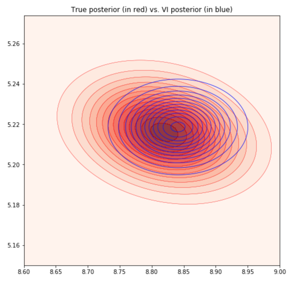
i.e. factorizes completely completely over each dimension. It turns out that this restriction significantly impacts the quality of inferences made using VI, because it cannot model any correlations between dimensions. Hence, no solution of VI will ever be able to resemble the true posterior $p$ if there is any correlation present in it. In contrast, other inferential methods such as MCMC guarantee samples from the true $p$ in the asymptotic limit. We can illustrate this shortcoming of mean-field VI with a simple Bayesian linear regression example. It can be shown that the posterior for this case is a Gaussian with non-zero diagonal terms in the covariance matrix. We show the fitting of this posterior with mean-field VI in Figure 1.

Figure 1: True posterior vs. VI posterior for Bayesian linear regression

As expected, the true posterior $p$ has a slope due to the non-zero diagonals, something which our mean-field assumed $q$ could never capture. There are also two other commonly experienced problems (Turner & Sahani, 2011):

Under-estimation of the variance of the posterior. This is observed in the above plot where our $q$ is more concentrated.
Biases in the MAP solution of parameters. This is observed in the above plot where our learned $\mu$ for $q$ does not coincide perfectly with the true $\mu$ for $p$.

These issues mean that the subsequent decisions we make using our VI solution could be biased and have incorrect uncertainty estimates. In fields such as medical operations, these could have dire consequences.

Alternatives

There are a number of proposals for rich posterior approximations that have been explored, but there are some limitations :

Structured mean-field : Instead of assuming fully factorized posteriors, this assumes that the distribution factorizes into a product of tractable distributions, such as trees or chains (Shukla, Shimazaki, & Ganguly, 2019). While this allows for the modeling of some correlations, the subsequent optimization becomes too complex for any realistic applications.
Mixture model : This specifies the approximate posterior as a mixture model, and hence captures multi-modality well (Jordan et al., 1999). However, this limits the potential scalability of VI since it requires evaluation of the log-likelihood and its gradients for each mixture component per parameter update, which is typically computationally expensive.

Normalizing Flows

A normalizing flow describes the transformation of a probability density through a series of invertible mappings, making the initial simple density ‘flow’ through the mappings and result in a more complex distribution (Tabak & Turner, 2013). These mappings can be shown to preserve the PDF normalization property :

$\int_\mathbf{z}q_k(\mathbf{z}_k)d\mathbf{z}_k = 1$

at each stage $k$ of the flow, resulting in a valid density at the end.

We will consider the simple case of Planar flows, which introduces enough complexity in the approximate posterior $q$ for many applications. This uses an invertible and smooth mapping $f:\mathbb{R}^d \rightarrow \mathbb{R}^d$. We can think of these Planar flows as a sequence of expansions and contractions on the initial density $q_0$. If we use this to transform a random variable $\mathbf{z} \sim q(\mathbf{z})$, the resulting $\mathbf{z}^\prime = f(\mathbf{z})$ can be shown to be distributed as :

$q(\mathbf{z}^\prime) = q(\mathbf{z})\left|\det\frac{\partial f^{-1}}{\partial \mathbf{z}^\prime}\right| = q(\mathbf{z})\left|\det\frac{\partial f}{\partial \mathbf{z}^\prime}\right|^{-1}$

Now, imagine applying this process multiple times to construct arbitrarily complex distributions. After $K$ such transformations on the initial $\mathbf{z}_0$, using the above equation, the resulting random variable

$\mathbf{z}_K = f_K\circ\cdots\circ f_1(\mathbf{z_0})$

has log density

$\log q_K(\mathbf{z}_K) = \log q_0(\mathbf{z}_0) - \sum_{k=1}^K \log\left|\det\frac{\partial f_k}{\partial \mathbf{z}_{k-1}}\right|$

This path formed by the distributions $q_1,\cdots,q_K$ is called a normalizing flow. Using the law of the unconscious statistician (Blitzstein & Hwang, 2014), we are able to compute expectations using the transformed density $q_k$ without explicity knowing it :

$\mathbb{E}_{q_k}\left[h(\mathbf{z})\right] = \mathbb{E}_{q_0}\left[h\left(f_k\circ f_{k-1}\circ\cdots\circ f_1(\mathbf{z}_0)\right)\right]$

Using this equation is one of the major innovations for using normalizing flows for VI, since we will need to eventually compute expectations under later flow distributions $q_k, k\in{1,\cdots K}$. However, since it is not always possible to sample $\mathbf{z}_k \sim q_k(\mathbf{z}_k)$ if $q_k$ becomes complex enough, this equation allows us to compute such expectations using $\mathbf{z}_0 \sim q_0$ where $q_0$ would be the simple starting distribution we select, e.g. an isotropic Gaussian.

Planar flows can be expressed as :

$f(\mathbf{z}) = \mathbf{z} + \mathbf{u}h(\mathbf{w}^\text{T}\mathbf{z} + b)$

where the parameters $\lambda = {\mathbf{w}\in\mathbb{R}^D, \mathbf{u}\in\mathbb{R}^D, b\in\mathbb{R}}$ and $h$ is a smooth non-linearity that is chosen to be $tanh$ for this flow. Note that we can write the derivative of the $h(\mathbf{w}^\text{T}\mathbf{z} + b)$ term using chain rule as :

$\psi(\mathbf{z}) = h^\prime(\mathbf{w}^\text{T}\mathbf{z} + b)\mathbf{w}$

Hence using the matrix determinant lemma,

$\left|\det\frac{\partial f}{\partial \mathbf{Z}}\right| = \left|\det\left(\mathbf{I} + \mathbf{u}\psi(\mathbf{z})^\text{T}\right)\right| = \left|1 + \mathbf{u}^\text{T}\psi(\mathbf{z})\right|$

The log density from above can thus be expressed as

$\log q_K(\mathbf{z}_K) = \log q_0(\mathbf{z}_0) - \sum_{k=1}^K \log\left|1 + \mathbf{u}_k^\text{T}\psi_k(\mathbf{z}_{k-1})\right|$

which only requires an analytical distribution expression for the simple $q_0$.

VI with Normalizing Flows

This paper proposes a technique to implement VI using Normalizing Flows. The main ideas from the authors are :

Specify the approximate posterior using normalizing flows that allows for construction of complex distributions by transforming a density through a series of invertible mappings. This provides a tighter, modified evidence lower bound (ELBO) with additional terms that have linear time complexity. This is in contrast with the alternative methods above which require more complex optimizations.
It can be shown that using VI with normalizing flows specifies a class of $q$ distributions that provide asymptotic guarantees, as opposed to naive mean-field VI.
This method is shown to systematically outperform other competing approaches for posterior approximation.

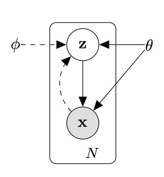
We will now provide deeper explanations of the above ideas. As an overview, we consider the general Variational Autoencoder (VAE) structure. A VAE is an unsupervised learning method that seeks to find a low-dimensional representation of usually high-dimensional data. For instance, if the observed data (denoted $\mathbf{X}$) is 100-dimensions, one might try to map those observed data into a latent space of 10 dimensions (where the latent variable is denoted $\mathbf{Z}$). This mapping is done through a simple neural network, called an inference or recognition network. Then, this latent representation $\mathbf{Z}$ can be used to generate new data by running the learned latent variables through a second neural network called a generative network. This process of mapping observed to latent variables and back to observed is characteristic of an autoencoder model. However, a variational autoencoder changes this paradigm. Rather than learning a single latent vector $\mathbf{z}_ n$ for each observed vector $\mathbf{x}_ n$, the inference network outputs the parameters of a distribution of possible $\mathbf{z}_ n$’s for each $\mathbf{x}_ n$. Typically, in order to make inference tractable, these parameters are the mean and variance of a diagonal gaussian. Another trick to optimize VAEs is amortisation. That is, rather than learning a set of $\mu$’s, $\sigma$’s, and flow parameters for each observation, we can instead notice that observed data points that are nearby in observed space should be similarly close in latent space. That means that we can instead learn a function $g_\phi(\mathbf{x})$, parameterised by $\phi$ that takes in observed data and outputs the mu, sigma, and flow parameters for those data. This is much computationall cheaper than the learning of explicit parameters for each data point. This amortisation is accomplished by the inference network itself. For more on variational autoencoders, see (Kingma & Welling, 2014) (https://arxiv.org/abs/1312.6114). This is summarized in the following (Pan, 2019):

\begin{align} z_n &\sim p_\theta(z), \; \mathbf{(prior)}\\ x_n &\sim p_\theta(x_n|z_n), \; \mathbf{(likelihood)} \end{align}

Hence we need to :

Learn $f_\theta$, the generative network, that will learn the mapping from latent variable $z_n$ to observed data $x_n$. Hopefully, we can learn to mimic the empirical distribution of observed data well.
Learn $g_\phi$, the inference network, that will learn the mapping from observed data $x_n$ to latent variable $z_n$. Hopefully, we can learn to infer the best approximation to the posterior of $z_n$ given an observation $x_n$.

These are summarized in the image below :

However, with normalizing flows, we can learn much more flexible families of distributions. This allows for more information to be encoded in otherwise highly compressed latent representations, meaning that we can potentially increase the ability of the autoencoder to faithfully reconstruct the observed data without sacrificing the compactnes and explainability of the latent representation. As per the standard variational formulation (Jordan et al., 1999), the marginal observed data likelihood can be bound as :

$\begin{aligned} \log p_\theta (\mathbf{x}) &= \log \int p_\theta (\mathbf{x}|\mathbf{z})p(\mathbf{z})d\mathbf{z}\\ &= \log \int \frac{q_\phi(\mathbf{z}|\mathbf{x})}{q_\phi(\mathbf{z}|\mathbf{x})}p_\theta (\mathbf{x}|\mathbf{z})p(\mathbf{z})d\mathbf{z}\\ &\geq -\mathbb{D}_{\text{KL}}\left[q_\phi(\mathbf{z}|\mathbf{x}) \middle\| p(\mathbf{z})\right] + \mathbb{E}_{q_\phi(z|x)}\left[\log p_\theta (\mathbf{x}|\mathbf{z})\right]\\ &= \mathbb{E}_{q_\phi(z|x)}\left[\log p(\mathbf{x}, \mathbf{z}) - \log q_\phi(\mathbf{z}|\mathbf{x})\right]\\ &= -\mathcal{F}(\mathbf{x}) \end{aligned}$

where we used Jensen’s to obtain the inequality. We hence have to minimize this free energy $\mathcal{F}(\mathbf{x})$.

We now integrate this with our normalizing flows formulation. As per the diagram above, we parameterize the overall VAE approximate posterior with a flow of length $K$ :

$q_\phi(\mathbf{z}|\mathbf{x}) := q_K(\mathbf{z}_K)$

The free energy now becomes :

$\begin{aligned} \mathcal{F}(\mathbf{x}) &= \mathbb{E}_{q_\phi(z|x)}\left[\log q_\phi(\mathbf{z}|\mathbf{x}) - \log p(\mathbf{x}, \mathbf{z})\right] \\ &= \mathbb{E}_{q_0(z_0)}\left[\log q_K(\mathbf{z}_K) - \log p(\mathbf{x}, \mathbf{z}_K)\right] \\ &= \mathbb{E}_{q_0(z_0)}\left[\log q_0(\mathbf{z}_0)\right] - \mathbb{E}_{q_0(z_0)}\left[\log p(\mathbf{x}, \mathbf{z}_K)\right]-\mathbb{E}_{q_0(z_0)}\left[\sum_{k=1}^K \log\left|1 + \mathbf{u}_k^\text{T}\psi_k(\mathbf{z}_{k-1})\right|\right] \end{aligned}$

where we used the normalizing flow log density derived above. We now have an objective function to minimize that only needs an analytical expression for the chosen simple distribution $q_0$, an analytical expression for the joint likelihood $p$ that depends on our model and the various flow parameters $\lambda$ that we want to learn. The generative network parameters $\theta$ are a part of the likelihood $p$ while the inference network parameters $\phi$ are the flow parameters $\lambda$ which is a part of the final summation term. We can also opt to learn the optimal parameters of the initial distribution $q_0$, which would be a part of the first term. Hence, optimizing $\mathcal{F}$ should allow us to learn the optimal $\theta, \phi$ as needed in VAEs. All the expectations can be computed using Monte Carlo estimation with $\mathbf{z}_0 \sim q_0$, something that we can easily sample. We are thus able to minimize the objective using any optimization package.